Genesis

A long time ago I discovered a wonderful book by Hal Abelson and Gerald Sussman called The Structure and Interpretation of Computer Programs. The book aims to introduce engineering students to computing using the Scheme programming language. It presents a wonderful view of programming; investigating a wide variety of interesting and practical examples, and even showing how a language like Scheme can be implemented.

At about the same I obtained access to one of the first releases of Rick Becker and John Chambers' New S language. I remember noticing both similarities and differences between S and Scheme. In particular, I remember that one day I wanted to show Alan Zaslavsky how you could use lexical scope to obtain own variables. I didn't have a copy of Scheme handy, so I tried to show him using S. My demonstration failed because of the differences in the scoping rules of S and Scheme. It left me thinking that there were useful additions which could be made to S.

Rather later, Robert Gentleman and I became colleagues at The University of Auckland. We both had an interest in statistical computing and saw a common need for a better software environment in our Macintosh teaching laboratory. We saw no suitable commercial environment and we began to experiment to see what might be involved in developing one ourselves.

It seemed most natural to start our investigation by working with a small Scheme-like interpreter. Because it was clear that we would probably need to make substantial internal changes to the interpreter we decided to write our own, rather than adopt one the many free Scheme interpreters available at the time. This is not quite as daunting a task as it might seem. The process is well mapped out in books such as that of Abelson-Sussman and that of Kamin. Having access to the source code of a number Scheme interpreters also helped with some of the concrete implementation details.

Our initial interpreter consisted of about 1000 lines of C code and provided a good deal of the language functionality found in the present version of R. To make the interpreter useful, we had to add data structures to support statistical work and to choose a user interface. We wanted a command driven interface and, since we were both very familiar with S, it seemed natural to use an S-like syntax.

This decision, more than anything else, has driven the direction that R development has taken. As noted above, there are quite strong similarities between Scheme and S, and the adoption of the S syntax for our interpreter produced something which "felt" remarkably close to S. Having taking this first step we found ourselves adopting more and more features from S.

Despite the similarity between R and S, there remain number of key differences. The two fundamental differences result from R's Scheme heritage.

• Memory Management: In R, we allocate a fixed amount of memory at startup and manage it with an on-the-fly garbage collector. This means that there is very little heap growth and as a result there are fewer paging problems than are seen in S.
• Scoping: In S, variables in functions are either local or global. In R we allow functions to access to the variables which were in effect when the function was defined; an idea which dates back to Algol 60 and found in Scheme and other lexically scoped languages. Consider the function definition in figure *. The function make.counter returns a value which is itself a function. This "inner function" increments the value of the variable total, and then returns the value of that variable. In S, the variable being manipulated is global. In R, it is the one which is in effect when the function is defined; i.e. it is the argument to make.counter. The effect is to create a variable which only the inner function can see and manipulate.

          > total <- 10
          > make.counter <-
          +   function(total = 0)
          +     function() {
          +       total <<- total + 1
          +      total
          +     }
          > counter <- make.counter()
          > counter()
          [1] 1
          > counter()
          [1] 2
          > counter()
          [1] 3
  

  A simple function demonstrating how the scoping rules in R differ from those of S.

   

  Generally, the scoping rules used in R have met with approval because they promote a very clean programming style. We have retained them despite the fact that they complicate the implementation of the interpreter.

The two differences noted above are of a very basic nature. In addition, we have experimented with a number of other features in R. A good deal of the experimentation has been with the graphics system (which is quite similar to that of S). Here is a brief summary of some of these experiments.

• Colour Model: R uses a device independent 24-bit model for colour graphics. Colours can be specified in a number of ways.
  1. By specifying the levels of red, green and blue primaries which make up the Colour. For example, the string "#FFFF00" indicates full intensity for red and green with no blue; producing yellow.
  2. By giving a colour name. R uses the colour naming system of the X Window System to provide about 650 standard colour names, ranging from the plain "red", "green" and "blue" to the more exotic "light goldenrod", and "medium orchid 4".
  3. As a index into a user settable colour table. This provides compatibility with the S graphics system.
• Line Texture Description: Line textures can also be specified in a flexible fashion. The specification can be:
  1. A texture name (e.g. "dotted").
  2. A string containing the lengths for the pen up/down segments which compose a line. For example, the specification "52" indicates 5 points (or pixels) with "pen down" followed by 2 with "pen up", with the pattern replicated for the length of the line.
  3. An index into a fixed set of line types, again providing compatibility with S.

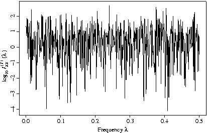
  A plot of the periodogram of a white-noise time series, showing the use of mathematical annotation.  

• Mathematical Annotation: Paul Murrell and I have been working on a simple way of producing mathematical annotation in plots. Mathematical annotation is produced by specifying an unevaluated R expression instead of a character string. For example,

  expression(x^2+1)

  can be used to produce the mathematical expression x^2+1 as annotation in a plot.

  The annotation system is relatively simple, and not designed to have the full capabilities of a system such as TeX. Even so, it can produce quite nice results. Figure * shows a simple example of a time series periodogram plot produced in R. The plot was produced with a single R command which used expression to describe the labels.

• Flexible Plot Layouts: A part of his PhD research, Paul Murrell has been looking at a scheme for specifying plot layouts. The scheme provides a simple way of specifying how the surface of the graphs device should be divided up into a number of rectangular plotting regions. The regions can be constrained in a variety of ways. Paul's original work was in Lisp, but he has implemented a useful subset to R.

These graphical experiments were carried out at Auckland, but others have also bound R to be an environment which can be used as a base for experimentation.

• Compilation: Luke Tierney has performed some experiments to see what kind of performance gains could be obtained by using byte-code compilation of R. His experiments indicated that a speed-up by a factor of 20 might be possible for some interpreted code. As yet, the internal data structures in R are probably not stable enough to make it worthwhile to follow up on this work.
• WWW Interface: Jeff Banfield has developed RWeb, which is a WWW based interface to R.
• Tcl/Tk Interface: Very recently Balasubramanian Narasimhan has begun looking into how Tcl/Tk might be used to add a fully graphical user interface to R.